Average temperatures: Climate California – Temperature, Rainfall and Averages
Temperature – US Monthly Average
Data Snapshots Image Gallery
Q:What was the average temperature?
A:
Colors show the average monthly temperature across each of the 344 climate divisions of the contiguous United States. Climate divisions shown in white or very light colors had average temperatures near 50°F. Blue areas on the map were cooler than 50°F; the darker the blue, the cooler the average temperature. Orange to red areas were warmer than 50°F; the darker the shade, the warmer the monthly average temperature.
Q:Where do these measurements come from?
A:
Temperature readings come from weather stations in the Global Historical Climatology Network. Scientists collect the highest and lowest temperature of the day at each station for the entire month. After they check data quality, they calculate the station’s monthly average and plot it on a gridded map. To fill the grid, a computer program applies a mathematical filter that accounts for the distribution of stations and the terrain. The monthly average temperature for each climate division is the average of all grid point values that fall within it.
Q:What do the colors mean?
A:
Shades of blue show climate divisions that had monthly average temperatures below 50°F. The darker the shade of blue, the lower the average temperature. Climate divisions shown in shades of orange and red had average temperatures above 50°F. The darker the shade of orange or red, the higher the average temperature. White or very light colors show climate divisions where the average temperature was near 50°F.
Q:Why do these data matter?
A:
Tracking average temperature in each of the 344 climate divisions of the contiguous United States gives scientists a way to monitor climate at a regional scale. Energy companies use this information to estimate demand for heating and air conditioning. Agricultural businesses also use these data to optimize timing of planting, harvesting, and putting livestock to pasture.
Q:How did you produce these snapshots?
A:
Data Snapshots are derivatives of existing data products: to meet the needs of a broad audience, we present the source data in a simplified visual style. This set of snapshots is based on climate division data (nClimDiv) produced by and available from the National Centers for Environmental Information (NCEI) – Weather and Climate. To produce our images, we invoke a set of scripts that access the source data and represent them according to our selected color ramps on our base maps.
References
NCEI Monthly National Analysis
U.S. Climate Divisions
Climate at a Glance – Data Information
Monitoring Global and U.S. Temperatures (FAQ)
- Data Provider
- National Centers for Environmental Information (NCEI) – Weather and Climate
- Source Data Product
- NCEI Climate at a Glance
- Access to Source Data
- Climate Division Data (nClimDiv)
- Reviewer
- Jake Crouch, National Centers for Environmental Information
We value your feedback
Help us improve our content
Your Email Address
Feedback
Security code
Get new captcha!
Statewide Average Weather for All Fifty U.
 S. States
This page compares the yearly average temperature and precipitation in all fifty U.S. states. It is based on the average temperature over the entire territory of the state between 1991–2020.
Select month: Entire Year\nJanuary\nFebruary\nMarch\nApril\nMay\nJune\nJuly\nAugust\nSeptember\nOctober\nNovember\nDecember
* Click column headers to sort.
| Alabama | 75.0 | 52.2 | 56.9 |
| Alaska | 35.5 | 20.4 | 37.6 |
| Arizona | 75.3 | 46.8 | 11.6 |
| Arkansas | 71.8 | 50.2 | 52.5 |
| California | 71.5 | 46.5 | 22.3 |
| Colorado | 60.0 | 32.4 | 18.0 |
| Connecticut | 60.0 | 39.8 | 48.7 |
| Delaware | 66.1 | 46.3 | 45. 9 9 |
| Florida | 81.9 | 60.9 | 54.4 |
| Georgia | 75.6 | 52.7 | 50.4 |
| Hawaii [1] | 80.4 | 66.6 | 43.2 |
| Idaho | 55.7 | 32.1 | 23.7 |
| Illinois | 62.7 | 42.6 | 40.7 |
| Indiana | 62.5 | 42.2 | 43.6 |
| Iowa | 58.5 | 38.1 | 35.6 |
| Kansas | 67.5 | 42.6 | 29.0 |
| Kentucky | 67.2 | 45.4 | 50.4 |
| Louisiana | 77.5 | 56.7 | 59.7 |
| Maine | 51.9 | 31.7 | 45.5 |
| Maryland | 65.4 | 45.4 | 45.2 |
| Massachusetts | 58.8 | 38.7 | 48.6 |
| Michigan | 55.0 | 35.3 | 33.9 |
| Minnesota | 51. 9 9 | 31.4 | 28.6 |
| Mississippi | 75.3 | 53.0 | 58.5 |
| Missouri | 66.0 | 44.5 | 43.5 |
| Montana | 54.7 | 30.4 | 18.9 |
| Nebraska | 61.9 | 36.9 | 24.2 |
| Nevada | 64.6 | 37.4 | 10.2 |
| New Hampshire | 54.7 | 33.3 | 47.9 |
| New Jersey | 63.6 | 43.6 | 47.6 |
| New Mexico | 69.5 | 39.4 | 13.8 |
| New York | 55.9 | 36.1 | 43.5 |
| North Carolina | 70.5 | 48.6 | 50.8 |
| North Dakota | 52.2 | 29.8 | 18.8 |
| Ohio | 61.7 | 41.6 | 41.1 |
| Oklahoma | 72.3 | 48.3 | 36.4 |
| Oregon | 59.4 | 36.4 | 32. 1 1 |
| Pennsylvania | 59.7 | 39.2 | 45.0 |
| Rhode Island | 60.0 | 41.3 | 49.1 |
| South Carolina | 74.7 | 52.0 | 48.3 |
| South Dakota | 57.5 | 33.8 | 21.2 |
| Tennessee | 69.4 | 47.5 | 55.1 |
| Texas | 78.1 | 53.5 | 28.6 |
| Utah | 62.0 | 36.4 | 13.5 |
| Vermont | 53.4 | 32.7 | 46.0 |
| Virginia | 66.9 | 45.1 | 45.8 |
| Washington | 57.0 | 37.6 | 43.2 |
| West Virginia | 63.5 | 41.7 | 47.1 |
| Wisconsin | 54.0 | 33.7 | 34.1 |
| Wyoming | 55.2 | 29.3 | 16.0 |
Averages by month:
January |
February |
March |
April |
May |
June |
July |
August |
September |
October |
November |
December |
Year
1. Data for all states except Hawaii is calculated by the NOAA. For Hawaii, the number represents the average of 5 locations: Honolulu, Hilo, Molokai Airport, Lihue, and Kula Hospital at an elevation of 944 meters in Maui.
Scientists have calculated the average temperatures on Earth during the last glaciation – Nauka
TASS, August 27. Paleoclimatologists have found that during the last glacier advance, the average temperature on the Earth’s surface was about 9 °C. The researchers came to this conclusion after studying samples of ancient ice and deposits on the walls of caves from the glaciation period. The results of the work were published in the scientific journal Nature.
“Our calculations show that at that time, temperatures on Earth decreased by an average of 6.1 ° C. In the context of current global warming, this means that if there is twice as much carbon dioxide in the atmosphere, then the temperature on the planet will increase by 3, 4 ° C. This is more than previous estimates associated with the last glacial maximum, but fits well with the predictions of conventional climate models,” the researchers write. nine0003
The last ice age in Earth’s history began about 2.6 million years ago. Its main feature is that the area of glaciation and the temperature of the Earth’s surface during the entire period were not constant. Due to sharp cooling and warming, glaciers advanced and retreated every few tens of thousands of years.
The last “thaw” of this kind occurred about 13 thousand years ago and continues to this day, and the last advance of glaciers, the so-called glacial maximum, began about 33 thousand years ago and peaked 26 thousand years ago. Scientists are studying the consequences of these events in the hope of understanding how long the current warm period will last and how the Earth’s climate has changed during this time. nine0003
Climatologists led by Associate Professor at the University of Arizona (USA) Jessica Tierney have received the first accurate estimates of how much the average temperature on Earth dropped during the last glacial maximum. These data, as the researchers explain, are important in order to understand how temperatures on Earth change with sharp changes in the concentration of carbon dioxide or the area of ice cover, which happened both then and now.
To obtain such information, scientists have collected samples of deposits from the walls of several dozen caves scattered around the world, as well as deposits of ancient ice from Greenland and Antarctica. After analyzing their isotopic and chemical composition, paleoclimatologists have found out how much the temperatures in these corners of the Earth have fallen or risen over the past 30 thousand years, and used them to create a model of the planet’s climate during the last glacial maximum. nine0003
“Climate models predict that at high latitudes, global warming will be faster and stronger. This will be especially pronounced in the Arctic. Something similar, but the opposite in meaning, happened during the last glacial maximum,” Tierney explained.
According to her, then the temperature in the temperate latitudes of the Earth fell by 3-5 °C, while in the subpolar regions it decreased by 14 °C. A similar cold snap occurred in Europe, Canada and the northern United States. This explains why glaciers at that time covered almost all of their territory. nine0003
With this data, scientists calculated how sensitive the Earth’s climate is to sudden changes in the concentration of greenhouse gases in the atmosphere and the area of the polar ice caps. As Tierney and her colleagues hope, this updated data will help their colleagues more accurately predict how the planet’s climate will change in the coming decades and centuries, and develop optimal methods to combat global warming.
TS.3.1.1 Global Mean Temperatures – AR4 WGI Technical Summary
ContentsTSTS.3TS.3.1TS.3.1.1
2005 and 1998 were the warmest years on record for global surface air temperatures since 1850. Surface temperatures increased in 1998 due to a major El Niño event in 1997-1998, but there was no such strong anomaly in 2005. Eleven of the last 12 years (1995-2006) – with the exception of 1996 – are among the 12 warmest years on record since 1850. {3.2}
The global mean surface temperature has increased, especially since 1950 years. Due to additional warm years, the updated 100-year trend (1906-2005) of 0.74°C ± 0.18°C exceeds the 100-year warming trend recorded at the time of the TAR (1901-2000) of 0 .6°C ± 0.2°C. The total temperature rise from 1850-1899 to 2001-2005 is 0.76°C ± 0.19°C. The warming rate averaged over the last 50 years (0.13°C ± 0.03°C per decade) is almost double that of the last 100 years). All three different global estimates show consistent warming trends. There is also consistency between individual land and ocean datasets, and between sea surface temperatures (SSTs) and nighttime sea air temperatures (see Figure TS.6). {3.2}
Global temperature trends
TS.6. (Top) Characteristics of linear global temperature trends over the period 1979-2005 estimated at the surface (left) and from satellites in the troposphere (right). Areas with incomplete data are highlighted in gray. (Bottom) Annual average global temperatures (black dots) fitted with a straight line from the data. The left axis shows temperature anomalies relative to the 1961-1990 average, while the right axis shows actual temperature estimates (all values are in °C). Linear trends are shown over the past 25 (yellow), 50 (orange), 100 (purple), and 150 (red) years. The smoothed blue curve shows decadal variations (see Appendix 3.A), with decadal 90% margin of error, indicated by the pale blue bar above this line. Total temperature increase from 1850-1899 to 2001-2005 is 0.76°C ± 0.19°C. {FAQ 3.1, fig. 1.}
Recent research confirms that the impacts of urbanization and land-use change on global temperature are negligible (less than 0.006°C per decade over land and zero over oceans) in terms of hemispheric and continental averages. All observations should be checked for data quality and consistency to eliminate potential bias. The real but local effects of urban areas are taken into account in the land temperature datasets used. The effects of urbanization and land use do not play a role in the wide-scale ocean warming that is evident from observations. There is growing evidence that urban heat island effects also influence precipitation, cloud cover and diurnal temperature range (DST). {3.2}
{3.2}
The global average DST has stopped decreasing. The TAR noted a decrease in DST during the period 1950-1993. by approximately 0.1°C per decade. Updated observations show that the DST has not changed from 1979 to 2004, as both daytime and nighttime temperatures increased at the same rate. Trends are highly variable from region to region. {3.2}
New analyzes of radiosonde and satellite measurements of lower and middle troposphere temperatures show warming rates that are broadly consistent with each other and with surface temperature rise rates within their respective uncertainties over periods of 1958-2005 and 1979-2005. This largely eliminates the contradiction noted in the TAR (see Figure TS.7). Radiosonde datasets are noticeably less spatially comprehensive than surface temperature data, and there is growing evidence that some radiosonde datasets are unreliable, especially in the tropics. Inconsistencies remain between the various tropospheric temperature trends estimated with satellite microwave sensing equipment (MSU) and advanced microwave sensing since 1979 years, and all of them probably still contain residual errors.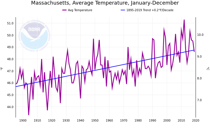 However, since the TAR, trend estimates have improved significantly and differences between datasets have narrowed due to adjustments for satellite changes, lower orbit heights, and drift in local equator-crossing time (diurnal cycle effects). It turns out that the results of satellite measurements of tropospheric temperature are largely consistent with surface temperature trends, provided that the influence of the stratosphere on channel 2 of the ISYU is taken into account. Range across different global surface warming datasets since 1979 years is 0.16°C – 0.18°C per decade, compared to 0.12°C – 0.19°C per decade for the ISU tropospheric temperature estimates. It is likely that in the tropics there is increased warming with increasing height from the earth’s surface to most of the troposphere, a pronounced cooling in the stratosphere, and a trend towards a higher tropopause. {3.4}
Observed air temperatures
TS.7. Observed surface temperatures (D) and temperatures at heights – in the lower troposphere (C), in the middle and upper troposphere (B), in the lower stratosphere (A), shown as monthly average anomalies relative to the period 1979-1997 smoothed with a seven-month moving average filter.